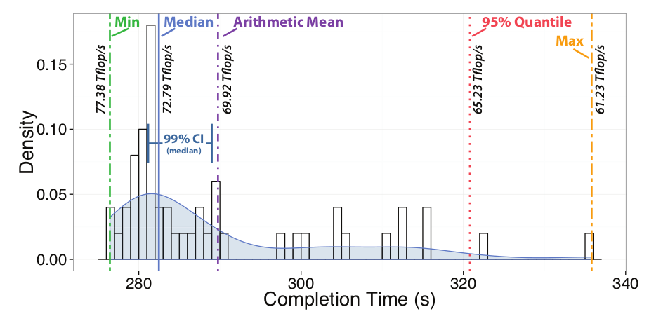
The following figure from the paper “Scientific Benchmarking of Parallel Computing Systems” shows the completion times for multiple identical runs of a tuned version of the high-performance Linpack (HPL) on the same system. It illustrates how important correct measurements are. Here, one may report 77.4 Tflop/s but when repeating the benchmark see as little as 61.2 Tflop/s. It suggests that one should use sound statistics when reporting any performance result.
Computer science is often about measuring computer systems. Be it time, energy, or performance, all these metrics are often non-deterministic in real computer systems and a single measurement may or may not provide a reliable result. So if you are not sloppy when measuring your system, you will measure several executions and report an aggregate measure such as the arithmetic or geometric average or the median. Well, but now the question is: “how many is several”? And this is where it gets less clear.
Typically, “several” is defined very informally, so if the measurement is cheap (such as a network latency measurement), it can be 1,000 or even 1,000,000. If it’s expensive (such as full-scale supercomputer runs), we’re very quickly back to a single measurement. But does it make sense to define the number of measurements based on the execution cost? Of course not — it should depend on the variability of the data! Who would have thought that …?
Unfortunately, most benchmarkers do not take the data variability into account at all in practice. Why not? Isn’t that somewhat clear that one needs to? Yes, it is, but it’s also hard! But actually, it’s not that hard if one knows some basic statistics. The simplest way is to check if one has enough measurements for a given variability in the result. But how to assess the variability? Well, one needs to look at some samples — ah, a catch 22? I need samples to know how many samples I need? Yes, that is true — in fact, the more samples I have, the higher my confidence in the variability and the correctness of my reported number.
A simple technique to assess the confidence of my measurement (we are simplifying this somewhat here) is to compute the confidence interval. Confidence Intervals (CIs)
are a tool to provide a range of values that include the true mean with a given probability p depending on the estimation procedure. So if the measurement is 1 second and the 95% CI is the range [0.9;1.1] then there is a 95% probability that the true mean is within that interval. There are two basic types of CIs: (1) confidence intervals around the mean assuming a normal distribution and (2) nonparametric confidence intervals around the median without assumptions on the distribution. The former CI one is simplest to compute: [mean-t(n-1,p/2)/sqrt(n); mean+t(n-1,p/2)/sqrt(n)] where mean is the arithmetic mean, n is the number of samples, and t(x,p) is student’s t distribution with x degrees of freedom. So it’s easy to see that the interval quickly gets tighter when the number of samples grows. But which computing system generates measurements following a standard distribution, which means that it’s equally likely to become faster than slower. Well, my computers are certainly more often becoming slower than faster leading to a right-skewed distribution.
So how do we get to confidence intervals of non-normally distributed measurements? Well, first of all, if the data is not normally distributed, the average makes little sense as it will be skewed as well. So one usually reports the median (the n/2-th element in the sorted set of all n measurements) as the most likely value to be observed in practice. But how to get to our confidence interval? Since we cannot assume any distribution of the values, we work on the sorted set of measurements and call the rank-i value the ith value in the set. Now we identify rank floor((n-z(p/2)*sqrt(n))/2) to ceil(1+(n+z(p/2)*sqrt(n))/2) as the conservative CI which is commonly asymmetric as well.
So ok, we can now compute this CI as statistical measure of certainty of our reported median. Median what? Don’t we like averages? Well, again, averages are not too useful for non-normally distributed data *unless* you care about only an accumulation of many measurements, i.e., you only want to know how expensive 1,000 iterations are and you do not care about every single one. Well, if this is the case, just measure the 1,000. If you’re well-versed in statistics, you will now recognize the connection to the Central Limit Theorem :-).
But now again, how many measurements do we actually need?? To answer this, we’d first need to define a needed level of certainty, for example 95%. Then, we define an accepted error in our reporting around the median, for example 1%. In other words, we would like to have enough measurements to be 95% sure that the real median is within 1% of our reported value. Hey, so we’re now back to a single reported value just together with a certainty! So how do we achieve this? Well, for normally distributed data in the case (1), one could compute the number of needed measurements. But that doesn’t work with real computers, so let’s skip this here. In the nonparametric case, no explicit formula is known to us, so we would need to recompute the confidence interval after each measurement (or a set of measurements) and we could stop measuring once the 95% CI is within the 1% interval around the mean.
Wow, so now we know how to *really* measure and report performance! In fact, in practice, we often need less than 1,000 measurements to reach a tight interval with high confidence. So if they’re cheap, we can as well do them and check afterwards of the statistics make sense. But what if we are running out of benchmarking budget before we reach the required accuracy — for example, each measurement takes a day and we only have four days but after four days, the CI is still wider than we’d like it to be? Well, bad luck! In that case, we can only report the wide CI and leave it up wo the reader/observer to conclude if our measurements make sense in his context.
I wish you happy (and correct) measuring! Torsten Hoefler
This blog post summarizes a part of the paper “Scientific Benchmarking of Parallel Computing Systems” which appeared at IEEE/ACM Supercomputing 2015. The full paper provides more insight and references around this topic and also the equation for the number of measurements assuming a normal distribution. The paper also establishes more rules for sound performance analyses that I may blog on later. Spread the word and cite the paper if you find these rules useful :-).